Shalaila Haas

Part 1: ggseg visualization with Freesurfer data in R

Purpose of this post

I enjoy finding new ways to visualize data in a meaningful (and also aesthetically pleasing) way. Finding the right tools in order to get your message across adds value, but can be challenging. When I learned about this visualization toolbox with the multitude of options it has, I had to learn how to use it – and it’s actually quite simple!

The links to both the blog and GitHub pages below are extremely informative (so please also refer to them)! Here, I wanted to outline the installation process I used in order to get the program running in RStudio (Part 1) and provide some examples of things I have done with the toolbox to potentially spark some inspiration (Part 2)!

Getting Started

Source

All the credits for this awesome toolbox go to Dr. Athanasia Mowinckel & Dr. Didac Vidal Pineiro at the Center for Lifespan Changes in Brain and Cognition, University of Oslo. Be sure to check out Dr. Mowinckel’s blog, which has a great overview of the different options available with the toolbox.

ggseg GitHub link: https://github.com/LCBC-UiO/ggseg

ggseg GitHub README.md: https://github.com/LCBC-UiO/ggseg/blob/master/README.md

Note: There seem to be some updates happening at the moment with the toolbox, so this may not work 100% for you, but it worked for me in May of 2020. Updates to come if this changes.

Compatibility – what I used

Operating System: Windows 10

R version: 4.0.0

RStudio version: 1.2.5033

Installation Guide

Libraries to install prior to ggseg

library(ggplot2)
library(devtools)
library(tidyselect)
library(magrittr)
library(rmarkdown)
library(stringr)
library(stringi)
library(tibble)
library(dplyr)
library(purrr)
library(pandocfilters)
library(tidyr)

If some libraries are missing, use the command below with the toolbox name within the quotes as shown for tidyr.

$> install.packages("tidyr")

Installing ggseg

On the GitHub website, they state to use:

$> install.packages("remotes")
remotes::install_github("LCBC-UiO/ggseg", build_vignettes = TRUE)

Currently, there is a bug that is being fixed in the program with the Vignettes, so you will need to modify the code until this is fixed to:

$> install.packages("remotes")
$> remotes::install_github("LCBC-UiO/ggseg", build_vignettes = FALSE)

Personally, for me, I found that devtools works for installing the program without any problems. So since I already installed devtools above, just enter the following in RStudio:

$> devtools::install_github("LCBC-UiO/ggseg", build_vignettes = FALSE)
$> library(ggseg)

This will take a little bit of time and install version 1.5.4. You should see this in your window as:

$> building 'ggseg_1.5.4.tar.gz'

Atlases

After installing ggseg, there are two default atlases pre-installed based on the default Freesurfer output from running recon -all:

  • Desikan-Killany cortical atlas (dk)
  • Subcortical segmentation atlas (aseg)

Additionally, the following atlases are available and the links show examples for how to use the atlases. These are beyond the scope of this post. I will focus just on the default atlases included in the package.

  • Yeo – both 7 and 17 network data
  • Desterieux – the 2009 atlas
  • Chen – both thickness and area maps
  • Schaefer – both 17 and 7 networks
  • Glasser – full atlas
  • JHU – white tract atlas
  • Tracula – white tract atlas
  • ICBM – white tract atlas
  • HO – Harvard-Oxford cortical (FSL)
  • DefaultExtra – extra 2d view for dk, p/a division

To install the extra atlases, first install ggsegExtra:

$> devtools::install_github("LCBC-UiO/ggsegExtra", build_vignettes = FALSE)
$> library(ggsegExtra)

To check to see which atlases are available enter the following command:

$> ggseg_atlas_repos()

Install the atlas you would like to use with the format below (using the Glasser atlas as an example):

$> devtools::install_github("LCBC-UiO/ggsegGlasser")
$> library(ggsegGlasser)

Now you should hopefully have ggseg installed and ready to go without any problems!
Installing Freesurfer Using Enhanced Mode Ubuntu 18.04 for Hyper-V on Windows 10

Prerequisites

Before getting started, I first installed Ubuntu within Hyper-V on my Windows 10 computer following the instructions below:
https://www.hanselman.com/blog/UsingEnhancedModeUbuntu1804ForHyperVOnWindows10.aspx

Link to FreeSurfer installation page

While the link below is extremely well-written and helpful, I noticed a few steps during my installation process using Ubuntu for Hyper-V that required additional steps, not listed on the page. This is meant to help others using the same system that I am with the installation procedure – described in detail below. https://surfer.nmr.mgh.harvard.edu/fswiki/DownloadAndInstall

Installation Steps

1. Download Freesurfer

Download FreeSurfer for Linux from the download page while logged into your Ubuntu VM

File to download: freesurfer-Linux-centos6_x86_64-stable-pub-v6.0.0.tar.gz

Link to download (you may need to be logged into your Gmail account in order to download the file): https://surfer.nmr.mgh.harvard.edu/pub/dist/freesurfer/6.0.0/freesurfer-Linux-centos6_x86_64-stable-pub-v6.0.0.tar.gz

2. Change Permissions

You will need to make sure you have permissions to write into /usr/local/ which is where you will unpack the FreeSurfer package.

$> sudo chmod -R 777 /usr/local/   

3. Unpack FreeSurfer Package

Unpack the package making sure you are in the directory where you saved the package. For me this was:

$> cd /home/shaas/Downloads
$> tar -C /usr/local -xzvf freesurfer-Linux-centos6_x86_64-stable-pub-v6.0.0.tar.gz

4. Install additional necessary packages

$> sudo apt-get -y install bc binutils libgomp1 perl psmisc sudo tar tcsh unzip uuid-dev vim-common libjpeg62-dev 

5. Setup & Configuration

To begin using FreeSurfer, you need to open a terminal window and define and environment variable called FREESURFER_HOME which is set to the location FreeSurfer was installed, and then source the setup script. Sourcing FreeSurfer needs to be done every time you open a new terminal window. Or, you can add the two lines below to your default setup file (.bashrc or .cshrc) and FreeSurfer will be sourced automatically every time you open a new window.

## bash
$> export FREESURFER_HOME=/usr/local/freesurfer
$> source $FREESURFER_HOME/SetUpFreeSurfer.sh

If done correctly, you should see output similar to this:

Setting up environment for FreeSurfer/FS-FAST (and FSL)
FREESURFER_HOME /usr/local/freesurfer
FSFAST_HOME     /usr/local/freesurfer/fsfast
FSF_OUTPUT_FORMAT nii
SUBJECTS_DIR    /usr/local/freesurfer/subjects
MNI_DIR         /usr/local/freesurfer/mni

6. Get a license to use Freesurfer

A license key must be obtained to make the FreeSurfer tools operational. Obtaining a license is free and comes in the form of a license.txt file. Once you obtain the license.txt key file, copy it to your FreeSurfer installation directory. This is also the location defined by the FREESURFER_HOME environment variable.

Get license here: https://surfer.nmr.mgh.harvard.edu/registration.html

Once downloaded in Ubuntu, copy to folder where your FreeSurfer is:

$> cp /home/shaas/Downloads/license.txt /usr/local/freesurfer 

7. Additional items to install

$> sudo apt-get update
$> sudo apt-get upgrade
$> sudo apt-get install libtool autoconf build-essential pkg-config automake tcsh

First teaching experience

Last Monday, I was given the opportunity to take over the second half of the course my supervisor is teaching for the Neuro-Cognitive Psychology Master program.

The course is titled: Neuroimaging in Psychosis and At Risk Mental State

Description: This course enable students to engage in understanding structural and functional brain changes in psychiatric disorders, especially in psychosis and prodromal stage of psychosis (at risk mental state).  An integrative approach in prediction and staging of psychosis consisting of brain imaging, neuropsychological and clinical routine is introduced to students. In the first part of the course students are strongly encouraged to discuss “real” clinical cases and gain basic knowledge in the field of neuroimaging in psychosis. In the second part of the course students join the data acquisition which already takes place within the framework of EU funded project PRONIA, which is aiming at facilitating the targeted prevention of psychoses. Furthermore, multi-center project PRONIA is working on optimizing candidate biomarkers for the prediction and staging of psychoses and generating a prognostic system that generalizes well across mental health services. This course will try to complement course N in it’s second part- students will analyze resting-state data in practical sessions using various Matlab toolboxes. At the end of the course students should be able to use a novel platform of modern psychiatry which provides a deeper understanding of clinical and cognitive features of psychosis and how they relate to brain changes in different stages of illness.

Some of the reading provided by the course includes:

  • Yung, A., Phillips L. , Yuen, H. & McGorry,P. (2004). Risk factors for psychosis in an ultra high-risk group: psychopathology and clinical features. Schizophrenia Research, 67(2-3), 131-42.
  • Koutsouleris N., Meisenzahl E., et al. (2009). Use of neuroanatomical pattern classification to identify subjects in at-risk mental states of psychosis and predict disease transition. Archives of General Psychiatry, 66(7),700-12.
  • Falkenberg, I., Kircher, T., & Krug, A. (2014). Neuroimaging in Schizophrenia. In MRI in Psychiatry (pp. 249-274). Springer Berlin Heidelberg.

After the students have spent some weeks covering varying topics within the course by preparing presentations for the other students, and then discussing the topics further – they had the opportunity to integrate all of this knowledge with an exercise. We watched an interview that my supervisor had conducted with a patient who had provided consent to do so, but remained fully anonymous to anyone watching the video. It was depicting the manner in which the interviews we conduct with patients generally occurs. It covers the types of questions we ask along with the formulations for the types of symptoms that come up in this At-Risk Mental State for psychosis. This patient expressed her feelings and described her experiences over the last years with a focus on the more recent changes.

We would watch a little clip for approximately 10 minutes at a time and then discuss her symptoms, and the students had an opportunity to try to discern her symptoms into an educated idea of what it was she might be diagnosed with. It was a somewhat complex example, as her symptoms were very multifaceted. There were aspects of personality disorder, social phobia/anxiety, paranoia and suspisciousness just to name a few.

It was a rewarding experience seeing the way the students engaged with these ideas and applied the knowledge they have accumulated throughout the course.

The papers that were included in the course to build this baseline knowledge include:

  • Pantelis, C., Yücel, M., Wood, S. J., Velakoulis, D., Sun, D., Berger, G., … & McGorry, P. D. (2005). Structural brain imaging evidence for multiple pathological processes at different stages of brain development in schizophrenia. Schizophrenia Bulletin, 31(3), 672-696.
  • van den Heuvel, M. P., & Fornito, A. (2014). Brain networks in schizophrenia. Neuropsychology review, 24(1), 32-48.
  • Benetti, S., Pettersson-Yeo, W., Allen, P., Catani, M., Williams, S., Barsaglini, A., … & Mechelli, A. (2013). Auditory verbal hallucinations and brain dysconnectivity in the perisylvian language network: a multimodal investigation.Schizophrenia bulletin, sbt172.
  • Zarogianni, E., Moorhead, T. W., & Lawrie, S. M. (2013). Towards the identification of imaging biomarkers in schizophrenia, using multivariate pattern classification at a single-subject level. NeuroImage: Clinical, 3, 279-289.
  • Wolfers, T., Buitelaar, J. K., Beckmann, C. F., Franke, B., & Marquand, A. F. (2015). From estimating activation locality to predicting disorder: A review of pattern recognition for neuroimaging-based psychiatric diagnostics.Neuroscience & Biobehavioral Reviews, 57, 328-349.
  • Satterthwaite, T. D., Vandekar, S. N., Wolf, D. H., Bassett, D. S., Ruparel, K., Shehzad, Z., … & Gur, R. E. (2015). Connectome-wide network analysis of youth with psychosis-spectrum symptoms. Molecular psychiatry.
  • Gur, R. C., Calkins, M. E., Satterthwaite, T. D., Ruparel, K., Bilker, W. B., Moore, T. M., … & Gur, R. E. (2014). Neurocognitive growth charting in psychosis spectrum youths. JAMA psychiatry, 71(4), 366-374.
  • Roiser, J. P., Howes, O. D., Chaddock, C. A., Joyce, E. M., & McGuire, P. (2013). Neural and behavioral correlates of aberrant salience in individuals at risk for psychosis. Schizophrenia bulletin, 39(6), 1328-1336.
  • Subramaniam, K., Luks, T. L., Fisher, M., Simpson, G. V., Nagarajan, S., & Vinogradov, S. (2012). Computerized cognitive training restores neural activity within the reality monitoring network in schizophrenia. Neuron, 73(4), 842-853.
  • Modinos, G., Renken, R., Shamay-Tsoory, S. G., Ormel, J., & Aleman, A. (2010). Neurobiological correlates of theory of mind in psychosis proneness.Neuropsychologia, 48(13), 3715-3724.

All in all it was a great experience – especially coming from someone who hasn’t much of an opportunity independently keeping other students engaged.

Meta-analysis Tools

Seed-based d Mapping

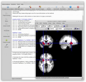
sdm_screenshot

Introduction

Seed-based d Mapping (formerly “Signed Differential Mapping”) is a statistical technique for meta-analyzing studies on differences in brain activity or structure which used neuroimaging techniques such as fMRI, VBM, DTI or PET. The methods have been fully validated in several studies (see references below), and meta-analyses using this method have been already published at the highest quality journals.

The method

An introduction of the method can be found in the SDM Reference Manual.

Briefly, some of the features are:

  • Possibility of combining studies from which only peak coordinates are available with studies from which SPM t-maps are available, highly increase the power of the meta-analysis.
  • Use of specific masks correlation templates for fMRI, PET, gray matter, white matter, fractional anisotropy, TBSS and cerebrospinal fluid to account for the anisotropy in the spatial covariance of the brain, highly increasing the accuracy of the recreation of the effect size maps.
  • Accounting for peaks’ effect-size and signed maps to counteract positive and negative differences.
  • Weighting the calculations for intra-study variance (i.e. studies with large sample sizes and/or lower error contribute more), inter-study heterogeneity and other optional weights.
  • Use of the random-effects general linear models to allow meta-analytical comparisons between groups, meta-regressions and use of covariates.
  • Complementary analyses such as exploration of heterogeneity (by means of heterogeneity maps, subgroup analyses and meta-regressions) and jackknife analyses (to assess thereplicability of the results)

Other useful tools within the website: